データ解析のための統計モデリング入門 一般化線形モデル(GLM) 読書メモ２

このブログ記事は『データ解析のための統計モデリング入門』（久保拓弥　著、岩波書店）という、とても分かりやすい統計モデリングの入門書を、さらに分かりやすくするために読書メモをまとめたものです。 今回は第３章、一般化線形モデル(GLM)についてのまとめの二回目です。 この章にはポアソン回帰の例が載っています。 本の中で使われているサンプルデータがここで公開されているので、解説されている通りにポアソン回帰をやってみました。 コードはRで書きました。

d <- read.csv("data3a.csv")
cat("summary of input data\n")
summary(d)

fit <- glm(y ~ x, data = d, family = poisson)

b1 <- fit$coefficients[1]
b2 <- fit$coefficients[2]

cat("\nlink function\n")
cat("exp(", b1, " + ", b2, "x)\n")

linkFunction <- function(x) {
exp(b1 + b2 * x)
}

ps <- 0:20
xl <- "y"
yl <- "probability"
legends <- c("x = 0","x = 5","x = 10", "x = 15", "x = 20")
pchs <- c(0, 5, 10, 15, 20)
title <- paste("lambda = exp(", b1, "+", b2, "x)")
plot(0, 0, type = "n", xlim = c(0, 20), ylim = c(0.0, 0.25), main = title, xlab = xl, ylab = yl)
for (x in seq(0, 20, by = 5)) {
d <- function(y) {
dpois(y, lambda = linkFunction(x))
}
lines(ps, d(ps), type = "l")
points(ps, d(ps), pch = x)
}
legend("topright", legend = legends, pch = pchs)

実行するとポアソン回帰を行い、得られる分布をプロットしてくれます。 実際にポアソン回帰をやっているコードは以下の部分です。

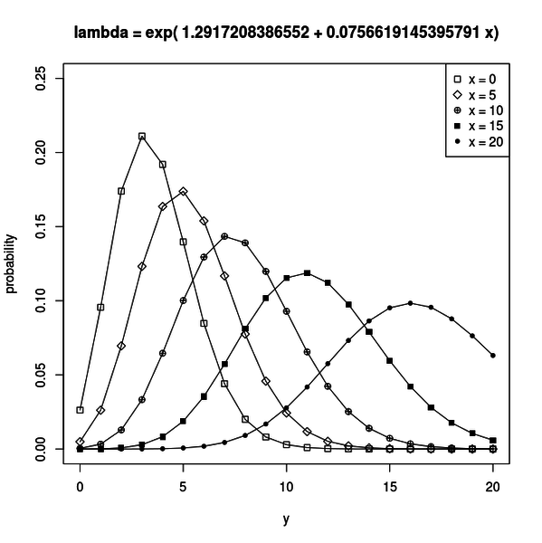
fit <- glm(y ~ x, data = d, family = poisson)

b1 <- fit$coefficients[1]
b2 <- fit$coefficients[2]

`b1` と `b2` が最尤推定されたパラメータです。 推定された結果は `b1 = 1.291721` 、 `b2 = 0.07566191` でした。 これらのパラメータが得られればリンク関数 `λ = exp(b1 + b2 x)` が得られるので、説明変数 `x` に対して `y` がどのような平均 `λ` でポアソン分布するかが分かります。 その分布は下図のようになります。 グラフを見ると `x` が大きくなるにしたがって `y` の分布が大きな値をとるように移動しているのが分かります。 これは、推定されたパラメータのうち、 `b2` が正だからです。 サンプルデータの `x` と `y` には正の相関があるのですね。