データ解析のための統計モデリング入門 GLMの尤度比検定と検定の非対称性 読書メモ5

このブログ記事は『データ解析のための統計モデリング入門』（久保拓弥　著、岩波書店）という、とても分かりやすい統計モデリングの入門書を、さらに分かりやすくするために読書メモをまとめたものです。 今回は第５章、GLMの尤度比検定と検定の非対称性についてのまとめの五回目です。 この章では尤度比検定などについて説明がされています。 尤度比検定の手法の一つとしてパラメトリックブートストラップ法が説明されています。 なので、パラメトリックブートストラップ法でどのようにデータがシミュレートされているか見るためのコードを用意しました。 コードはRで書きました。

linkFunction <- function(b1, b2) {
function(x) {
exp(b1 + b2 * x)
}
}

createData <- function(n, b1, b2) {
x <- runif(n, 1, 20)
y <- rpois(n, lambda = linkFunction(b1, b2)(x))
data.frame(x, y)
}

plotGraph <- function(data, fit1, fit2, title) {
plot(data$x, data$y, type = "p", main = title, xlab = "x", ylab = "y")
lines(0:20, linkFunction(fit1$coefficient[1], 0)(0:20), lty = "solid")
lines(0:20, linkFunction(fit2$coefficient[1], fit2$coefficient[2])(0:20), lty = "dashed")
nl <- paste0("y = exp(", round(fit1$coefficient[1], 3), ")")
xl <- paste0("y = exp(", round(fit2$coefficient[1], 3),
" + ", round(fit2$coefficient[2], 3), " * x)")
legend("topleft", legend = c(nl, xl), lty = c("solid", "dashed"))
}

bootstrap <- function(b1) {
simulatedData <- createData(100, b1, 0)
fit1 <- glm(formula = y ~ 1, family = poisson, data = simulatedData)
fit2 <- glm(formula = y ~ x, family = poisson, data = simulatedData)
fit1$deviance - fit2$deviance
}

for(i in 1:10) {
expData <- createData(20, 0.1, 0.07)
fit1 <- glm(formula = y ~ 1, family = poisson, data = expData)
fit2 <- glm(formula = y ~ x, family = poisson, data = expData)
dev <- fit1$deviance - fit2$deviance

P <- mean(replicate(1000, bootstrap(fit1$coefficient[1])) > dev)
title <- paste("P value", P)
plotGraph(expData, fit1, fit2, title)
}

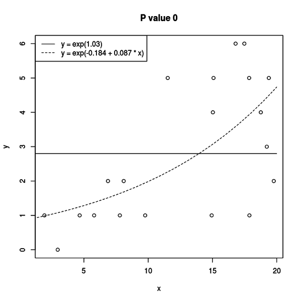
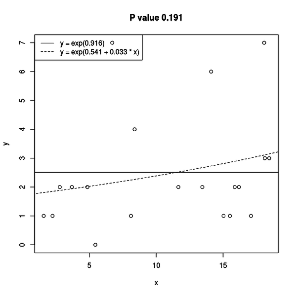
コードを実行するとグラフが10枚プロットされます。 それぞれにポアソン回帰で使われるデータと、推定されたモデルをプロットしてあります。 あと、パラメトリックブートストラップ法でP値を計算してタイトルに入れてあります。 典型的には下図のようなグラフがプロットされます。 ですが、時々は下図のようなグラフがプロットされます。 有意水準として5%を設定するなら、P値が0.05以上だと帰無仮説を棄却できません。 棄却できる時は対立仮説は帰無仮説とはだいぶ形の違う曲線になりますが、棄却できない時は直線に近い形になるのが分かります。 データは `x` に相関のある分布から生成されていますが、たまたまデータが偏っていると最尤推定で `x` と相関のないようなパラメータを推定してしまう場合があるわけですね。