データ解析のための統計モデリング入門 GLMの応用範囲をひろげる 読書メモ8
2017年 05月 09日
このブログ記事は『データ解析のための統計モデリング入門』(久保拓弥 著、岩波書店)という、とても分かりやすい統計モデリングの入門書を、さらに分かりやすくするために読書メモをまとめたものです。
今回は第6章、GLMの応用範囲をひろげるについてのまとめの八回目です。
この章では様々なタイプのGLMについて説明がされています。
その中でガンマ回帰について説明がされています。
なので、いろいろなパラメータについてガンマ回帰のモデルをプロットしてくれるコードを用意しました。
コードはRで書きました。
linkFunction <- function(b1, b2) {
  function(x) {
    exp(b1 + b2 * log(x))
  }
}

distribution <- function(x, s, linkFunction) {
  l <- match.fun(linkFunction)
  function(y) {
    dgamma(y, shape = s, rate = s / l(x))
  }
}

xs <- c(0.1, 1.0, 2.0, 3.0, 4.0)
ys <- seq(0.5, 10.0, by = 0.5)
pchs <- 1:5
xl <- "y"
yl <- "Probability"
legends <- paste0("x = ", xs)
for (b1 in seq(0.5, 2.5, by = 0.5)) {
  for (b2 in seq(0.5, 2.5, by = 0.5)) {
    for (s in 1:5) {
      l <- linkFunction(b1, b2)
      title <- paste0("shape = ", s, ", rate = ", s, " / exp(", b1, " + ", b2, "log(x))")
      plot(0, 0, type = "n", xlim = c(0, 10), ylim = c(0.0, 1.0), main = title, xlab = xl, ylab = yl)
      for (i in 1:5) {
        d <- distribution(xs[i], s, l)
        lines(ys, d(ys), type = "l")
        points(ys, d(ys), pch = pchs[i])
      }
      legend("topright", legend = legends, pch = pchs)
    }
  }
}
リンク関数は x の単調増加関数です。
コードでは以下の部分です。
linkFunction <- function(b1, b2) {
  function(x) {
    exp(b1 + b2 * log(x))
  }
}
これがガンマ分布の平均を与えます。
ガンマ分布にはshapeパラメータとrateパラメータがありますが、平均は shape / rate なのでリンク関数のパラメータだけを与えても、どんなガンマ分布になるか分かりません。
なので、リンク関数のパラメータ b1 と b2 の他にshapeパラメータも与えました。
コードを実行すると様々な b1 と b2 と shape の値に対してモデルをプロットします。
例えば下図のような図がプロットされます。
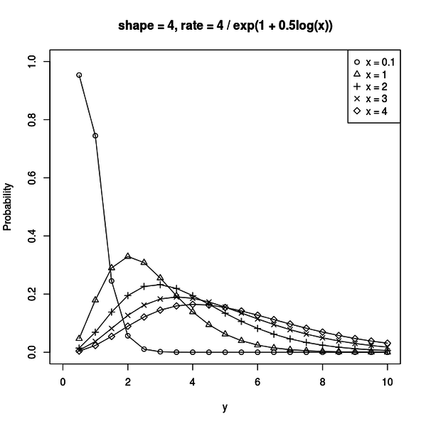
これは b1 = 1、b2 = 0.5、shape = 4 の場合です。
ガンマ分布の平均は shape / rate = exp(1 + 0.5 * log(x)) なので、rate = 4 / exp(1 + 0.5 * log(x)) になります。
平均が x の単調増加関数なので、x が大きな値を取るようになるほど y の分布も大きな値を取るように変化するのが分かります。

#人気の記事
#タグ